生态环境学报 ›› 2026, Vol. 35 ›› Issue (2): 190-198.DOI: 10.16258/j.cnki.1674-5906.2026.02.003
唐淑兰( ), 张旻曦
收稿日期:2025-05-08
修回日期:2025-11-04
接受日期:2025-11-20
出版日期:2026-02-18
发布日期:2026-02-09
通讯作者:
唐淑兰
作者简介:唐淑兰(1979年生),女,副教授,博士,研究方向为多源遥感数据时空融合、模式识别。E-mail: 2007010027@xaufe.edu.cn
基金资助:
TANG Shulan(), ZHANG Minxi
Received:2025-05-08
Revised:2025-11-04
Accepted:2025-11-20
Online:2026-02-18
Published:2026-02-09
摘要:
碳中和背景下陆地生态系统碳储量的精细化估测具有重要意义。为更精确地利用多源遥感影像调查陆地生态系统碳储量情况,该文提出融合高分1号(GF-1)多尺度特征及哨兵1号(Sentinel-1)结构特征的土地利用分类及碳储量估测方法。对GF-1经特征向量主成分分析的主分量影像进行小波包变换,依据代价函数选出最优小波包树,提取多尺度特征,再结合植被指数特征、Sentinel-1结构特征构造分类向量,利用随机森林(RF)筛选特征完成土地利用分类,最后基于InVEST模型估测碳储量。结果表明:1)GF-1光谱及小波包纹理融合Sentinel-1结构特征后,各土地利用分类总体精度可达92.46%,Kappa为0.91,估测的碳储量值为31.27 Tg,与实测碳储量值相比总体误差为0.81%;2)分类后各土地利用类型中,林地、住宅、水域、耕地、道路、园地、其他未利用土地占比分别为83.29%、2.32%、1.38%、4.44%、1.29%、6.42%、0.86%,对应的碳储量贡献占比分别为91.53%、0.03%、0.08%、2.77%、0.01%、5.50%、0.08%;3)该文方法较仅用GF-1光谱特征估测碳储量的误差降低了3.09%。可见,光学影像经最优小波包变换提取多尺度特征,再结合Sentinel-1的垂直特征,细化了地物分类,提高了碳储量的估测精度。该方法可为碳储量的遥感估测提供借鉴。
中图分类号:
唐淑兰, 张旻曦. 结合GF-1多尺度特征与Sentinel-1结构特征的土地利用分类及碳储量估测[J]. 生态环境学报, 2026, 35(2): 190-198.
TANG Shulan, ZHANG Minxi. Land Use Classification and Carbon Storage Estimation Based on GF-1 Multi-scale Features and Sentinel-1 Structural Features[J]. Ecology and Environmental Sciences, 2026, 35(2): 190-198.

图1 研究区位置
Figure 1 Location of the studied area
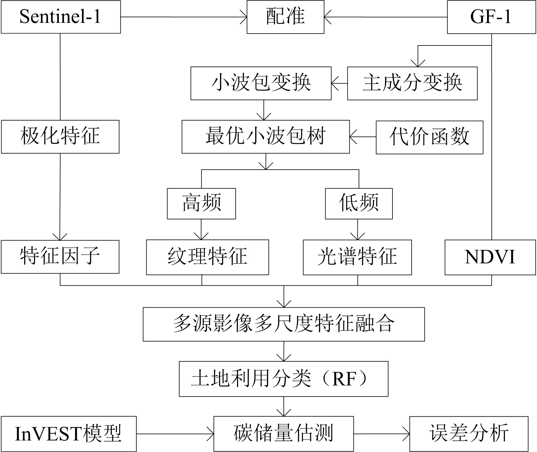
图2 结合GF-1多尺度特征与Sentinel-1结构特征的碳储量估测
Figure 2 Carbon storage estimation process combining GF-1 multiscale features and Sentinel-1 structural features
| 影像 | 特征 | 遥感特征因子 |
|---|---|---|
| Sentinel-1 | 后向散射系数 | $V(\mathrm{VV}), V(\mathrm{VH}), V(\mathrm{VV} / \mathrm{VH}), V_{[(\mathrm{VH}-\mathrm{VV}) /(\mathrm{VH}+\mathrm{VV})]}$ |
表1 Sentinel-1影像提取的遥感特征因子
Table 1 Remote sensing feature factors extracted from Sentinel-1 images
| 影像 | 特征 | 遥感特征因子 |
|---|---|---|
| Sentinel-1 | 后向散射系数 | $V(\mathrm{VV}), V(\mathrm{VH}), V(\mathrm{VV} / \mathrm{VH}), V_{[(\mathrm{VH}-\mathrm{VV}) /(\mathrm{VH}+\mathrm{VV})]}$ |
| 土地利用类型 | 碳密度/(t∙hm−2) | |||
|---|---|---|---|---|
| Cabove, i | Cbelow, i | Csoil, i | Cdead, i | |
| 林地 | 9.07 | 24.79 | 16.87 | 2.00 |
| 住宅 | 0.53 | 0.00 | 0.00 | 0.00 |
| 水域 | 2.80 | 0.00 | 0.01 | 0.00 |
| 耕地 | 1.22 | 17.26 | 11.52 | 0.00 |
| 道路 | 0.46 | 0.00 | 0.00 | 0.00 |
| 园地 | 7.55 | 18.50 | 10.61 | 4.50 |
| 其他 | 1.30 | 0.00 | 3.14 | 0.00 |
表2 研究区碳密度
Table 2 Carbon density in the studied area
| 土地利用类型 | 碳密度/(t∙hm−2) | |||
|---|---|---|---|---|
| Cabove, i | Cbelow, i | Csoil, i | Cdead, i | |
| 林地 | 9.07 | 24.79 | 16.87 | 2.00 |
| 住宅 | 0.53 | 0.00 | 0.00 | 0.00 |
| 水域 | 2.80 | 0.00 | 0.01 | 0.00 |
| 耕地 | 1.22 | 17.26 | 11.52 | 0.00 |
| 道路 | 0.46 | 0.00 | 0.00 | 0.00 |
| 园地 | 7.55 | 18.50 | 10.61 | 4.50 |
| 其他 | 1.30 | 0.00 | 3.14 | 0.00 |
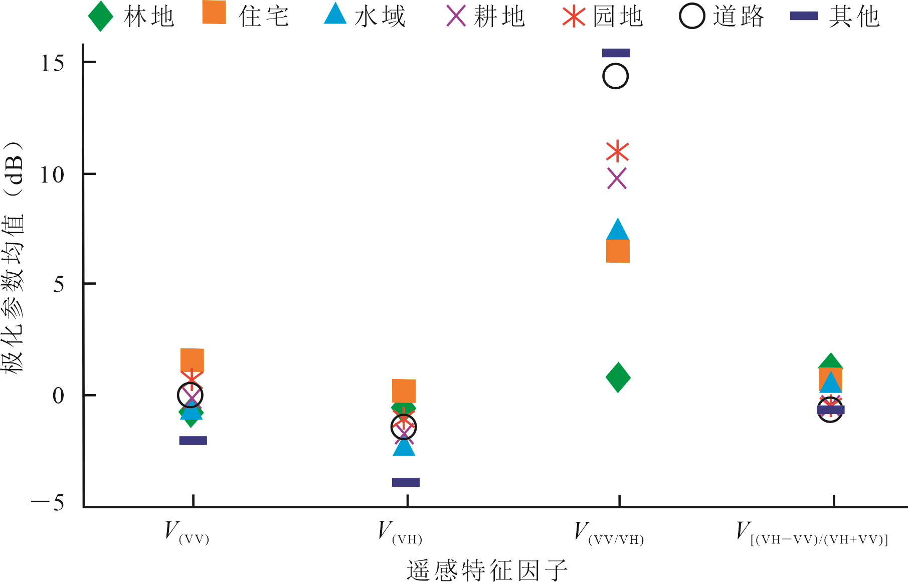
图3 SAR中各地类差异性
Figure 3 Differences of ground categories in SAR images
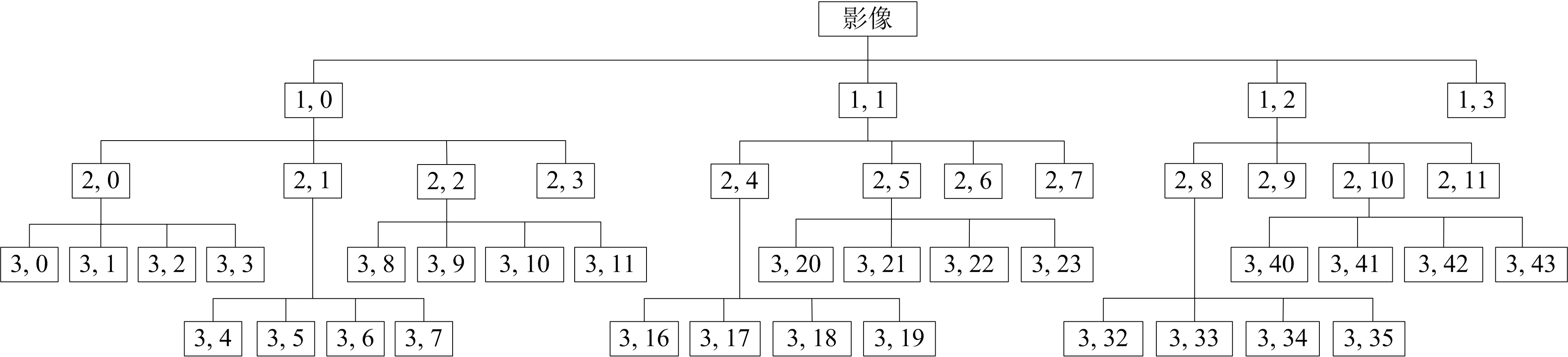
图4 最优小波包树
Figure 4 Optimal wavelet packet tree
| 节点号 | 节点熵值 | 节点号 | 节点熵值 | 节点号 | 节点熵值 |
|---|---|---|---|---|---|
| 1 | −26800.0 | 16 | −13.1 | 31 | −24.7 |
| 2 | −29200.0 | 17 | −2.6 | 32 | −3.3 |
| 3 | −100.0 | 18 | −32100.0 | 33 | −5.7 |
| 4 | −54.6 | 19 | −651.0 | 34 | −12.4 |
| 5 | −2.5 | 20 | −467.0 | 35 | −18.9 |
| 6 | −31100.0 | 21 | −102.0 | 36 | −3.9 |
| 7 | −316.0 | 22 | −118.0 | 37 | −5.2 |
| 8 | −190.0 | 23 | −148.0 | 38 | −16.9 |
| 9 | −22.2 | 24 | −18.6 | 39 | −3.2 |
| 10 | −55.1 | 25 | −34.1 | 40 | −12.9 |
| 11 | −40.2 | 26 | −80.7 | 41 | −4.1 |
| 12 | −3.7 | 27 | −15.9 | 42 | −2.7 |
| 13 | −4.3 | 28 | −71.5 | 43 | −1.1 |
| 14 | −36.8 | 29 | −23.4 | 44 | −6.8 |
| 15 | −4.0 | 30 | −22.1 | 45 | −2.7 |
表3 最优树各节点熵值
Table 3 The entropy values of each node in the optimal tree
| 节点号 | 节点熵值 | 节点号 | 节点熵值 | 节点号 | 节点熵值 |
|---|---|---|---|---|---|
| 1 | −26800.0 | 16 | −13.1 | 31 | −24.7 |
| 2 | −29200.0 | 17 | −2.6 | 32 | −3.3 |
| 3 | −100.0 | 18 | −32100.0 | 33 | −5.7 |
| 4 | −54.6 | 19 | −651.0 | 34 | −12.4 |
| 5 | −2.5 | 20 | −467.0 | 35 | −18.9 |
| 6 | −31100.0 | 21 | −102.0 | 36 | −3.9 |
| 7 | −316.0 | 22 | −118.0 | 37 | −5.2 |
| 8 | −190.0 | 23 | −148.0 | 38 | −16.9 |
| 9 | −22.2 | 24 | −18.6 | 39 | −3.2 |
| 10 | −55.1 | 25 | −34.1 | 40 | −12.9 |
| 11 | −40.2 | 26 | −80.7 | 41 | −4.1 |
| 12 | −3.7 | 27 | −15.9 | 42 | −2.7 |
| 13 | −4.3 | 28 | −71.5 | 43 | −1.1 |
| 14 | −36.8 | 29 | −23.4 | 44 | −6.8 |
| 15 | −4.0 | 30 | −22.1 | 45 | −2.7 |
| 土地利用类型 | 样本均值与背景均值的马氏距离 | ||
|---|---|---|---|
| M1 | M2 | M3 | |
| 林地 | 45.12 | 155.96 | 34.78 |
| 住宅 | 90.79 | 94.88 | 67.89 |
| 水域 | 216.53 | 220.27 | 168.65 |
| 耕地 | 121.08 | 176.78 | 102.43 |
| 道路 | 86.82 | 71.02 | 55.88 |
| 园地 | 115.18 | 125.73 | 81.77 |
| 其他 | 34.34 | 79.61 | 52.65 |
表4 各层样本均值与背景均值的分离度
Table 4 Separation degree between sample mean and background mean at each layer
| 土地利用类型 | 样本均值与背景均值的马氏距离 | ||
|---|---|---|---|
| M1 | M2 | M3 | |
| 林地 | 45.12 | 155.96 | 34.78 |
| 住宅 | 90.79 | 94.88 | 67.89 |
| 水域 | 216.53 | 220.27 | 168.65 |
| 耕地 | 121.08 | 176.78 | 102.43 |
| 道路 | 86.82 | 71.02 | 55.88 |
| 园地 | 115.18 | 125.73 | 81.77 |
| 其他 | 34.34 | 79.61 | 52.65 |
| 样本 | 林地 | 住宅 | 水域 | 耕地 | 道路 | 园地 | 其他 |
|---|---|---|---|---|---|---|---|
| 数量 | 29113 | 2816 | 1001 | 2674 | 845 | 2598 | 654 |
表5 样本数据集
Table 5 Sample data sets
| 样本 | 林地 | 住宅 | 水域 | 耕地 | 道路 | 园地 | 其他 |
|---|---|---|---|---|---|---|---|
| 数量 | 29113 | 2816 | 1001 | 2674 | 845 | 2598 | 654 |
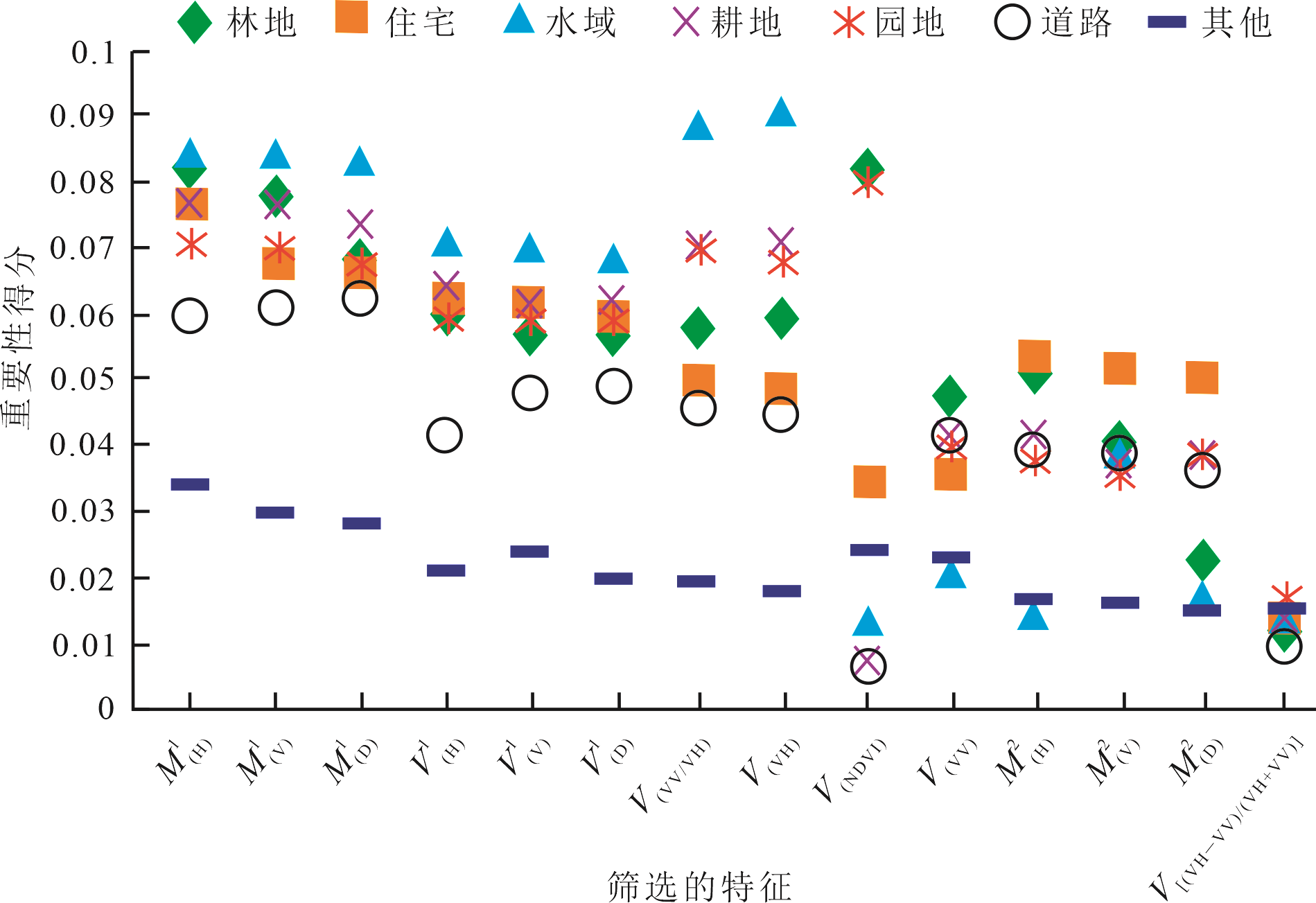
图5 特征重要性排名
Figure 5 Ranking of feature importance

图6 土地利用分类结果 1-耕地集中区域;2-园地集中区域;3-林地集中区域
Figure 6 Classification results of land use
| 精度及Kappa系数 | 土地利用类型 | ||||||
|---|---|---|---|---|---|---|---|
| 林地 | 住宅 | 水域 | 耕地 | 园地 | 道路 | 其他 | |
| 生产者精度(PA)/% | 98.24 | 93.78 | 91.36 | 99.13 | 98.10 | 61.69 | 87.70 |
| 用户精度(UA)/% | 99.34 | 99.23 | 85.40 | 98.67 | 86.93 | 81.56 | 99.57 |
| 总体精度(OA)/% | 92.46 | ||||||
| Kappa系数 | 0.91 | ||||||
表6 分类精度
Table 6 Classification accuracy
| 精度及Kappa系数 | 土地利用类型 | ||||||
|---|---|---|---|---|---|---|---|
| 林地 | 住宅 | 水域 | 耕地 | 园地 | 道路 | 其他 | |
| 生产者精度(PA)/% | 98.24 | 93.78 | 91.36 | 99.13 | 98.10 | 61.69 | 87.70 |
| 用户精度(UA)/% | 99.34 | 99.23 | 85.40 | 98.67 | 86.93 | 81.56 | 99.57 |
| 总体精度(OA)/% | 92.46 | ||||||
| Kappa系数 | 0.91 | ||||||
| 土地利用类型 | 林地 | 住宅 | 耕地 | 水域 | 园地 | 道路 | 其他 |
|---|---|---|---|---|---|---|---|
| 林地 | 93.856 | 0.000 | 0.001 | 0.021 | 3.622 | 0.945 | 0.045 |
| 住宅 | 0.000 | 91.014 | 2.528 | 2.840 | 0.000 | 0.359 | 0.001 |
| 耕地 | 0.088 | 1.179 | 75.953 | 2.290 | 0.750 | 3.727 | 0.011 |
| 水域 | 0.045 | 6.453 | 6.831 | 83.123 | 0.068 | 8.857 | 0.079 |
| 园地 | 5.693 | 0.000 | 7.018 | 1.048 | 93.718 | 14.378 | 0.032 |
| 道路 | 0.001 | 0.173 | 1.245 | 4.121 | 0.601 | 67.895 | 0.001 |
| 其他 | 0.317 | 0.443 | 0.972 | 3.861 | 0.040 | 0.277 | 99.834 |
表7 分类混淆累计百分比
Table 7 Cumulative percentage of classification confusion
| 土地利用类型 | 林地 | 住宅 | 耕地 | 水域 | 园地 | 道路 | 其他 |
|---|---|---|---|---|---|---|---|
| 林地 | 93.856 | 0.000 | 0.001 | 0.021 | 3.622 | 0.945 | 0.045 |
| 住宅 | 0.000 | 91.014 | 2.528 | 2.840 | 0.000 | 0.359 | 0.001 |
| 耕地 | 0.088 | 1.179 | 75.953 | 2.290 | 0.750 | 3.727 | 0.011 |
| 水域 | 0.045 | 6.453 | 6.831 | 83.123 | 0.068 | 8.857 | 0.079 |
| 园地 | 5.693 | 0.000 | 7.018 | 1.048 | 93.718 | 14.378 | 0.032 |
| 道路 | 0.001 | 0.173 | 1.245 | 4.121 | 0.601 | 67.895 | 0.001 |
| 其他 | 0.317 | 0.443 | 0.972 | 3.861 | 0.040 | 0.277 | 99.834 |

图7 基于G+W+S分类结合InVEST模型的碳储量估测结果
Figure 7 Carbon storage statistical results based on G+W+S classification combined with InVEST model
| 不同遥感数据的碳储量估测法 | 碳储量/Tg | 误差/% |
|---|---|---|
| G | 32.23 | 3.90 |
| G+W | 32.01 | 3.19 |
| G+W+S | 31.27 | 0.81 |
表8 不同遥感数据碳储量估测误差对比
Table 8 Comparison of carbon storage estimation errors for different remote sensing data
| 不同遥感数据的碳储量估测法 | 碳储量/Tg | 误差/% |
|---|---|---|
| G | 32.23 | 3.90 |
| G+W | 32.01 | 3.19 |
| G+W+S | 31.27 | 0.81 |
| 碳储量估测方法 | 碳储量/Tg | 误差/% |
|---|---|---|
| G+W+S | 31.27 | 0.81 |
| RF | 31.90 | 2.84 |
| KNN | 32.05 | 3.32 |
表9 与其他碳储量估测模型对比
Table 9 Comparison with other carbon storage estimation models
| 碳储量估测方法 | 碳储量/Tg | 误差/% |
|---|---|---|
| G+W+S | 31.27 | 0.81 |
| RF | 31.90 | 2.84 |
| KNN | 32.05 | 3.32 |
| [1] |
ARÉVALO P, BACCINI A, WOODCOCK C E, et al., 2023. Continuous mapping of aboveground biomass using Landsat time series[J]. Remote Sensing of Environment, 288: 113483.
DOI URL |
| [2] |
CHEN G B, SUN Z W, ZHANG L, 2020. Road identification algorithm for remote sensing images based on wavelet transform and recursive opera tor[J]. IEEE Access, 8: 141824-141837.
DOI URL |
| [3] | CARCARRA-BES V, PARDINI M, CHOI C, et al., 2021. Tandem-X and Gedi Data Fusion for a Continuous Forest Height Mapping at Large Scales[J]. IEEE International Geoscience and Remote Sensing Symposium IGARSS, 2021: 796-799. |
| [4] | DONG L F, DU H Q, HAN N, et al., 2020. Application of convolutional neural network on lei bamboo Above-Ground-Bio-mass (AGB) estimation using worldview-2 [J]. Remote Sensing, 12(6): 958. |
| [5] | HONG D F, GAO L R, HANG R L, et al., 2022. Deep encoder-decoder networks for classification of hyperspectral and LiDAR data[J]. IEEE Geoscience and Remote Sensing Letters, 19: 1-5. |
| [6] |
LI Q S, WONG F, FUNG T, 2021. Mapping multi-layered mangroves from multispectral, hyperspectral, and LiDAR data[J]. Remote Sensing of Environment, 258(3): 112403.
DOI URL |
| [7] |
LECHNER M, DOSTÁLOVÁ A, HOLLAUS M, et al., 2022. Combination of Sentinel-1 and Sentinel-2 Data for tree species classification in a central european biosphere reserve[J]. Remote Sensing, 14(11): 2687.
DOI URL |
| [8] |
QIAN S, ZHOU Q B, WU W B, et al., 2017. Mapping regional cropping patterns by using GF-1 WFV sensor data[J]. Journal of Integrative Agriculture, 16(2): 337-347.
DOI URL |
| [9] |
QIN Y W, XIAO X M, WIGNERON J P, et al., 2022. Large loss and rapid recovery of vegetation cover and aboveground biomass over forest areas in Australia during 2019-2020[J]. Remote Sensing of Environment, 278: 113087.
DOI URL |
| [10] |
SANKAR A S, NAIR S S, DHARAN V S, et al., 2015. Wavelet sub band entropy based feature extraction method for BCI[J]. Procedia Computer Science, 46: 1476-1482.
DOI URL |
| [11] |
WANG L A, ZHOU X D, ZHU X K, et al., 2016. Estimation of biomass in wheat using random forest regression algorithm and remote sensing data[J]. The Crop Journal, 4(3): 212-219.
DOI URL |
| [12] |
WANG L N, SUN M C, LIU J H, et al., 2020. A robust algorithm based on phase congruency for optical and SAR image registration in suburban areas[J]. Remote Sensing, 12(20): 3339.
DOI URL |
| [13] |
YE Y X, BRUZZONE L, SHAN J, et al., 2019. Fast and robust matching for multimodal remote sensing image registration[J]. IEEE Transactions on Geoscience and Remote Sensing, 57(11): 9059-9070.
DOI URL |
| [14] |
ZHANG B, FU H Q, ZHU J J, et al., 2021. A multi-baseline PolInSAR forest height inversion model based on Fourier - Legendre polynomials[J]. IEEE Geoscience and Remote Sensing Letters, 18(4): 687-691.
DOI URL |
| [15] | 陈日东, 林什全, 潘国英, 等, 2019. 天堂山林场森林地上生物量及碳储量的遥感估算模型构建[J]. 林业与环境科学, 35(3): 71-77. |
| CHEN R D, LIN S Q, PAN G Y, et al., 2019. Remote sensing model for forest above-ground biomass and carbon storage in Tiantang Mountain forest farm[J]. Forestry and Environmental Science, 35(3): 71-77. | |
| [16] | 陈松, 孙华, 吴童, 等, 2020. 基于Sentinel-2与机载激光雷达数据的误差变量联立方程组森林蓄积量估测研究[J]. 中南林业科技大学学报, 40(12): 44-53. |
| CHEN S, SUN H, WU T, et al., 2020. Study on the forest volume inversion based on the simultaneous equations of error variables of Sentinel-2 and airborne Lidar data[J]. Journal of Central South University of Forestry and Technology, 40(12): 44-53. | |
| [17] | 邵壮, 陈然, 赵晶, 等, 2022. 基于FLUS与InVEST模型的北京市生态系统碳储量时空演变与预测[J]. 生态学报, 42(23): 59-72. |
| SHAO Z, CHEN R, ZHAO J, et al., 2022. Spatio-temporal evolution and prediction of carbon storage in Beijing’s ecosystem based on FLUS and InVEST models[J]. Acta Ecologica Sinica, 42(23): 59-72. | |
| [18] | 杨潋威, 赵娟, 朱家田, 等, 2022. 基于PLUS 和InVEST 模型的西安市生态系统碳储量时空变化与预测[J]. 自然资源遥感, 34(4): 175-182. |
| YANG L W, ZHAO J, ZHU J T, et al., 2022. Spatial and temporal variation and prediction of ecosystem carbon storage in Xi’an based on PLUS and InVEST model[J]. Remote Sensing for Natural Resources, 34(4): 175-182. | |
| [19] | 张丹丹, 肖晨超, 魏丹丹, 等, 2022. 基于时空谱的生态保护修复工程碳汇遥感监测技术框架研究[J]. 航天返回与遥感, 43(6): 119-128. |
| ZHANG D D, XIAO C C, WEI D D, et al., 2022. Study on the technical framework of carbon sink monitoring for ecological protection and restoration projects based on spatial-temporal-spectral data[J]. Spacecraft Recovery & Remote Sensing, 43(6): 119-128. | |
| [20] | 朱建华, 田宇, 李奇, 等, 2023. 中国森林生态系统碳汇现状与潜力[J]. 生态学报, 43(9) : 1-15. |
|
ZHU J H, TIAN Y, LI Q, et al., 2023. The current and potential carbon sink in forest ecosystem in China[J]. Acta Ecologica Sinica, 43(9): 1-15.
DOI URL |
|
| [21] | 朱宁宁, 杨必胜, 董震, 2025. 森林植被碳储量的遥感估测流程与方法[J]. 遥感学报, 29(1): 134-146. |
|
ZHU N N, YANG B S, DONG Z, 2025. A novel framework for forest vegetation carbon stock estimation based on remote sensing[J]. National Remote Sensing Bulletin, 29(1): 134-146.
DOI URL |
| [1] | 王悦, 于福东, 张月, 相恒星, 焉恒琦, 毛德华. 基于PLUS-InVEST模型的东北黑土区景观格局与碳储量变化多情景模拟[J]. 生态环境学报, 2026, 35(2): 178-189. |
| [2] | 崔丽洋, 张磊, 贾夏, 赵永华, 穆琪, 司绍诚. 结合生态系统服务的南疆盐碱地土壤质量评价[J]. 生态环境学报, 2026, 35(2): 245-255. |
| [3] | 唐中奥, 淳祯杰, 段兴武, 张瑞环, 荣丽, 刘文旭. 模拟侵蚀对元江流域黄红壤土壤微生物和土壤有机碳的影响[J]. 生态环境学报, 2026, 35(1): 54-61. |
| [4] | 王国琳, 刘凯英, 宋宁宁, 刘君, 王芳丽, 王学霞, 宗海英, 李绍静. 盐碱土有机态氮组分对秸秆及秸秆生物炭输入的响应机理[J]. 生态环境学报, 2026, 35(1): 62-74. |
| [5] | 官金顺, 蒋新宇, 程炯, 陈三雄, 余世钦. 藻液添加提升稀土尾矿砂土壤碳氮固持能力[J]. 生态环境学报, 2025, 34(12): 1890-1899. |
| [6] | 夏依宁, 刘鹏翱, 何柯润, 田朝晖, 曾丽婷, 侯珂伦. 基于土地利用的长株潭都市圈碳储量时空格局与情景模拟[J]. 生态环境学报, 2025, 34(11): 1661-1674. |
| [7] | 王宗阳, 曾雪兰, 祝振昌, 郭芬, 罗丽娟, 张武英, 杜青平, 张远. 湛江市红树林植被及土壤碳密度空间分布及其驱动机制分析[J]. 生态环境学报, 2025, 34(11): 1705-1714. |
| [8] | 孔小云, 张永坤, 李润杰, 李颖, 林成清, 马占明, 辛继林, 杨晓璇, 党怡乐, 赵家艺, 冯玲正, 周燕. 湟水河流域耕地土壤团聚体有机碳空间变异特征及其驱动因素分析[J]. 生态环境学报, 2025, 34(11): 1715-1727. |
| [9] | 陈鑫怡, 毛雅若, 宋靓颖, 王童瑶, 李启权. 四川盆地耕地土壤全磷空间分布特征及其主控因素[J]. 生态环境学报, 2025, 34(10): 1569-1578. |
| [10] | 陈文涛, 肖娴, 张怡, 方国东, 涂保华, 陈宁. 稻田土壤羟基自由基生成机制及环境效应[J]. 生态环境学报, 2025, 34(10): 1654-1660. |
| [11] | 刘卿, 龚雨顺, 王伟, 方贤滔, 吴金水, 沈健林. 湖南典型茶园土壤有机碳及其组分时空特征[J]. 生态环境学报, 2025, 34(9): 1386-1397. |
| [12] | 吴桂玲, 吴晓晖, 欧为友, 周华坤, 马文文, 吉孝菲. 青海湖流域盐沼湿地典型植被群落土壤盐分离子分布研究[J]. 生态环境学报, 2025, 34(8): 1228-1239. |
| [13] | 李曼, 吴东丽, 何昊, 余慧婕, 赵琳, 刘聪, 胡正华, 李琪. 1990-2020年黄河流域碳储量时空演变及驱动因素研究[J]. 生态环境学报, 2025, 34(3): 333-344. |
| [14] | 申佳龙, 吴栎宏, 李林霜, 周远芳, 杨孝民. 典型喀斯特山地小流域土地利用类型对土壤有机碳组分及其固碳效应的影响[J]. 生态环境学报, 2025, 34(3): 358-367. |
| [15] | 贺宥文, 韩亚峰, 王旭刚, 孙丽蓉, 邢江冰, 曹晟源. 不同光照条件下农田湿地土壤碳排放的驱动因子差异[J]. 生态环境学报, 2025, 34(3): 391-400. |
| 阅读次数 | ||||||
|
全文 |
|
|||||
|
摘要 |
|
|||||