基于集合模型预测外来植物反枝苋的入侵趋势

doi:10.16258/j.cnki.1674-5906.2024.06.006

生态环境学报 ›› 2024, Vol. 33 ›› Issue (6): 888-899.DOI: 10.16258/j.cnki.1674-5906.2024.06.006

基于集合模型预测外来植物反枝苋的入侵趋势

杨乐^*()

兰州财经大学农林经济管理学院，甘肃兰州 730101

收稿日期:2024-03-01 出版日期:2024-06-18 发布日期:2024-07-30
通讯作者: *
作者简介:杨乐（1987年生），男，讲师，硕士研究生，主要研究方向为城市生态系统、生态城市规划、生态安全与保护方面的研究。E-mail: yangl@lzufe.edu.cn
基金资助:
国家社会科学基金项目(23BJY198);甘肃省教育厅高校教师创新基金项目(2024A-065)

Prediction of Invasive Trend of Alien Plant Amaranthus retroflexus Based on Ensemble Model

YANG Le^*()

School of Agricultural and Forestry Economics and Management, Lanzhou University of Finance and Economics, Lanzhou 730101, P. R. China

Received:2024-03-01 Online:2024-06-18 Published:2024-07-30

摘要/Abstract

摘要：

反枝苋（Amaranthus retroflexus L.）是一种入侵较早、分布范围广、危害程度严重的全国性分布恶性杂草。为了及时防控反枝苋，阻止或减缓进一步扩散蔓延，亟需明确其在中国的适宜生境及入侵趋势。基于296个分布点和32个环境变量，利用集合物种分布模型分析反枝苋在当前（1970—2000年）的潜在适生区，并预测未来（2021—2040年和2041—2060年）3种气候情景下（SSPs1-2.6、SSPs2-4.5和SSPs5-8.5）的分布格局，综合分析影响反枝苋地理分布的主要环境变量及入侵趋势。结果表明，1）通过3种模型精度评价指标（AUC、KAPPA和TSS），集合模型（EM）模拟和预测的结果最为准确，当前气候条件下反枝苋主要的潜在适生区分布在华北地区、华中地区、华东地区、华南地区、西南地区的东部、西北地区的南部和北部些许地区，分布面积为4.39×10⁶ km²。反枝苋的潜在分布重心位于陕西省延安市宜川县，地理坐标为110.32°E，36.13°N。2）影响反枝苋潜在分布的主要环境变量为年平均温度（Bio1）、土地利用覆盖（LUCC）、海拔（Altitude）和年降水量（Bio12）。3）在2030年和2050年的3种不同气候情景下，随着年份和排放情景的增加，反枝苋的总适生区面积均会增加，并且扩张区的面积远大于收缩区的面积，扩张面积的比率在11.2%—21.4%。反枝苋在未来均有向高纬度地区扩散的趋势，华北地区的东部和东北地区的南部扩散面积最为显著，西北地区的南部和西南地区的东部也在逐渐扩散。该研究结果将有助于对该物种入侵动态的早期预警，为及时采取防控措施阻止其传播扩散提供理论支持。

关键词: 反枝苋, 物种分布模型, 环境变量, 潜在适生区

Abstract:

Amaranthus retroflexus L. is a nationally distributed malignant weed with early invasion and wide distribution that causes serious harm. To promptly prevent and control A. retroflexus and effectively slow down or avoid its further spread, there is an urgent need to identify suitable habitats and invasion trends in China. Based on 296 distribution points and 32 environmental variables, using the meta-species distribution model, this study analyzed the potential suitable areas for A. retroflexus in the current period (1970-2000) and predicted the potential distribution pattern for A. retroflexus under three climate scenarios (SSPs1-2.6, SSPs2-4.5, and SSPs5-8.5) in the future (2021-2040 and 2041-2060). Furthermore, the main environmental variables and invasion trends affecting the geographical distribution of A. retroflexus were explored comprehensively. The results demonstrated that 1) through the three model accuracy evaluation indexes (AUC, KAPPA and TSS), the results of ensemble model (EM) simulation and prediction were proved to be the most accurate. Under the current climatic conditions, the main potential suitable areas of A. retroflexus were distributed in North China, Central China, East China, South China, the eastern part of Southwest China, and the southern and northern parts of Northwest China, with a distribution area of 4.39×10⁶ km². The potential distribution center of A. retroflexus is located in Yichuan County, Yan’an City, Shaanxi Province, with geographical coordinates of 110.32°E and 36.13°N. 2) The main environmental variables affecting the potential distribution of A. retroflexus included the annual average temperature (Bio1), land use and cover (LUCC), altitude, and annual precipitation (Bio12). 3) Under the three different climate scenarios in 2030 and 2050, with an increase in the year and emission scenario, the total suitable area of A. retroflexus will increase, and the expansion area will become much larger than the contraction area, accounting for 11.2%-21.4%. In addition, A. retroflexus will tend to spread to higher latitudes in the future. The diffusion areas in the eastern part of North China and southern part of Northeast China were the most significant. A. retroflexus also gradually spread in the southern part of Northwest China and the eastern part of Southwest China. Overall, the results of this study will contribute to the early warning of the invasion dynamics of this species and provide theoretical support for timely prevention and control measures to prevent further spread.

Key words: Amaranthus retroflexus, species distribution models, environmental variables, potential suitable areas

中图分类号:

Q948
X173

杨乐. 基于集合模型预测外来植物反枝苋的入侵趋势[J]. 生态环境学报, 2024, 33(6): 888-899.

YANG Le. Prediction of Invasive Trend of Alien Plant Amaranthus retroflexus Based on Ensemble Model[J]. Ecology and Environment, 2024, 33(6): 888-899.

图/表 14

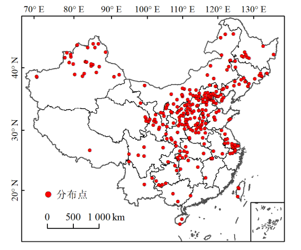
图1 反枝苋在中国的分布现状基于自然资源部标准地图服务网站2020年发布的GS（2020）4619号标准地图制作，底图边界无修改。下同

Figure 1 Distribution Status of A. retroflexus in China

表1 环境变量数据来源及其分辨率

Table 1 Environment variable data sources and their resolutions

数据名称	具体变量 (32个)	数据来源	数据分辨率
气候变量 (19个)	气温 (11个)、降水 (8个)	(http://www.worldclim.org)	2.5 arc-minutes
土壤属性变量 (9)	土壤有效含水量、含沙量、淤泥含量; 碎石体积百分比、粘土含量、有机碳含量; 土壤阳离子交换能力、土壤容重和酸碱度	https://www.fao.org/soils-porta
土地利用覆盖	土地利用覆盖类型	(http://www. resdc.cn)
地形变量 (3个)	海拔、坡向和坡度	(http://www.worldclim.org)
中国行政区划图	GS (2020) 4619号	(http://bzdt.ch.mnr.gov.cn/index.html)	矢量边界

表2 研究选用的10个环境变量

Table 2 10 environmental variables selected for the study

代码	描述
Bio1	年均温/℃
Bio2	平均气温日较差/℃
Bio3	等温性 (BIO2/BIO7) (×100)
Bio12	年降水量/mm
Bio15	降水量变异系数
Altitude	海拔/m
Aspect	坡向
LUCC	土地利用覆盖类型
T_SILT	淤泥含量
T_PH_H2O	酸碱度

图2 不同设置参数下模型表现 H是片段化（Hinge）、L是线性（Linear）、Q是二次型（Quadratic）、P是乘积型（Product）和T是阈值性（Threshold）

Figure 2 The model performance under different setting parameters

表3 11种模型的的KAPPA、TSS和AUC描述性统计

Table 3 Descriptive statistics of the KAPPA, TSS and AUC for 11 models

模型	AUC			KAPPA			TSS
模型	平均值	标准偏差	变异系数%	平均值	标准偏差	变异系数%	平均值	标准偏差	变异系数%
ANN	0.770	0.053	6.84	0.444	0.083	18.7	0.444	0.082	18.5
CTA	0.809	0.041	5.09	0.533	0.066	12.4	0.533	0.065	12.3
FDA	0.853	0.028	3.30	0.573	0.055	9.51	0.573	0.054	9.49
GAM	0.861	0.028	3.31	0.581	0.057	9.80	0.584	0.051	8.81
GBM	0.874	0.023	2.49	0.602	0.054	9.12	0.605	0.051	8.44
GLM	0.820	0.027	3.24	0.510	0.053	10.5	0.510	0.053	10.5
MARS	0.865	0.025	2.92	0.602	0.051	8.58	0.603	0.050	8.31
MaxEnt	0.834	0.052	6.36	0.580	0.086	14.9	0.579	0.086	14.9
RF	0.871	0.021	2.50	0.611	0.055	8.93	0.612	0.054	8.95
SRE	0.674	0.035	5.25	0.347	0.071	20.3	0.347	0.071	20.4
EM	0.887	0.010	1.14	0.645	0.006	1.05	0.645	0.007	1.13

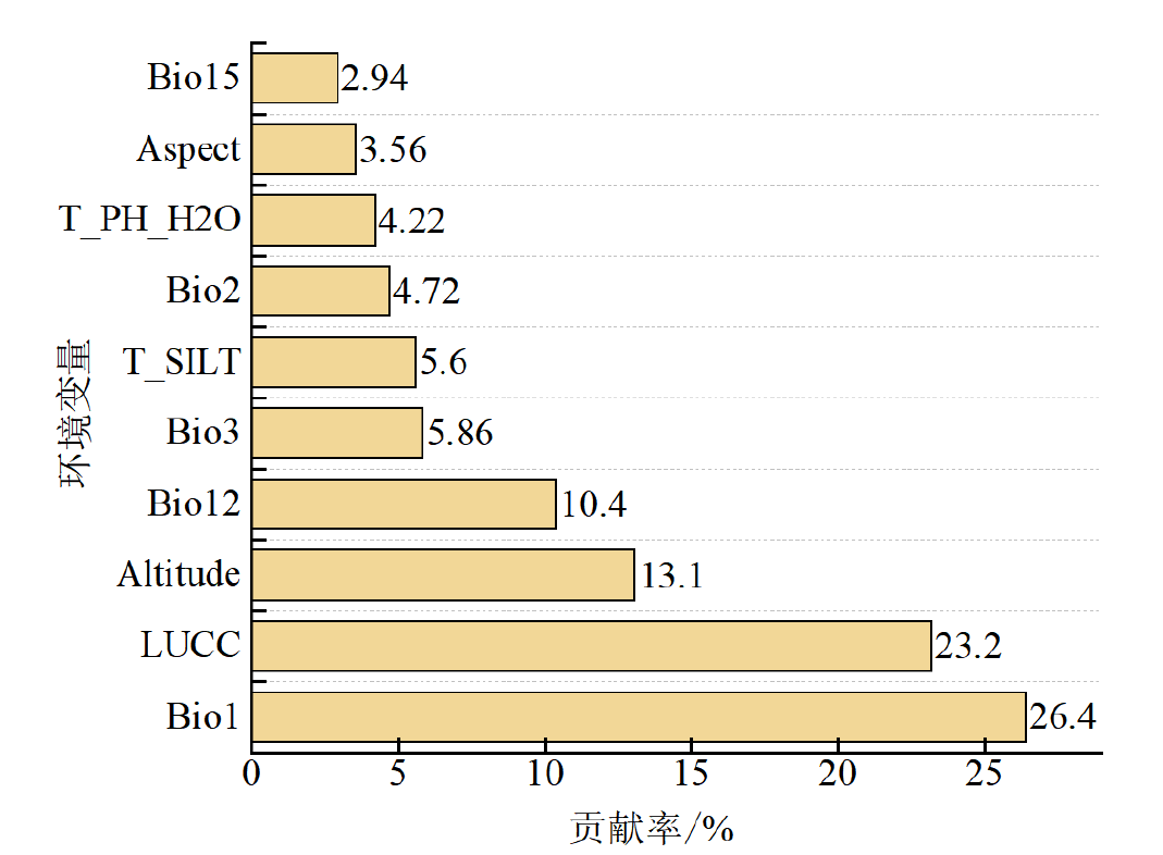
图3 参与建模的10个环境变量对反枝苋分布的贡献率

Figure 3 Contribution rate of 10 environmental variables involved in modeling to the distribution of A. retroflexus

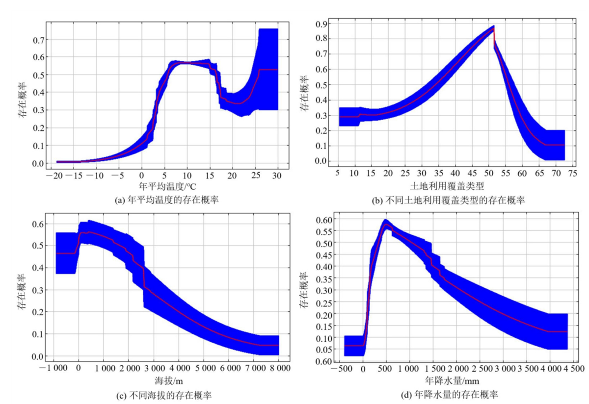
图4 反枝苋存在概率对主要环境变量的响应曲线

Figure 4 The response curve of A. retroflexus survival probability to dominant environmental factors

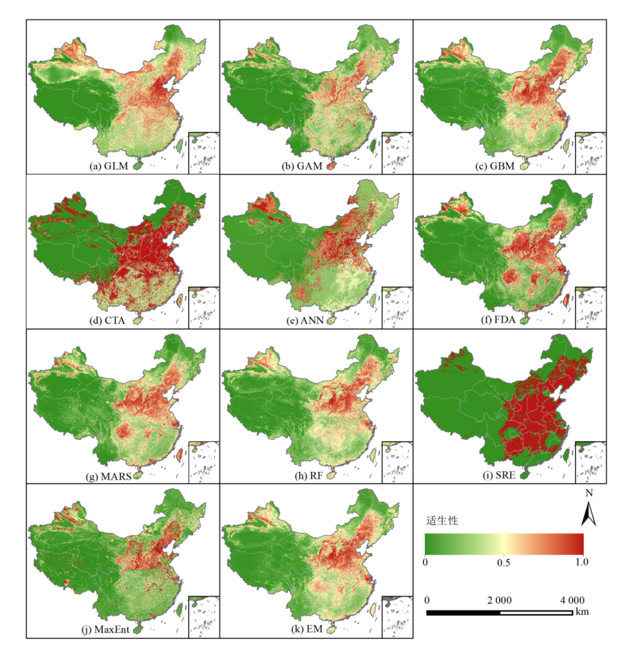
图5 11种物种分布模型模拟反枝苋的潜在适生区分布

Figure 5 Simulated potential suitable area distributions of A. retroflexus from eleven species distribution model

表4 不同时期反枝苋的适生区面积

Table 4 The suitable habitat area of A. retroflexus in different periods 106 km2

时期	高适生区	中适生区	低适生区	总适生区
当前	0.884	1.30	2.21	4.39
2030s, SSPs1-2.6	0.962	1.41	2.32	4.69
2030s, SSPs2-4.5	0.920	1.44	2.39	4.75
2030s, SSPs5-8.5	0.975	1.55	2.42	4.94
2050s, SSPs1-2.6	0.930	1.43	2.35	4.70
2050s, SSPs2-4.5	0.925	1.54	2.43.	4.89
2050s, SSPs5-8.5	0.935	1.67	2.46	5.07

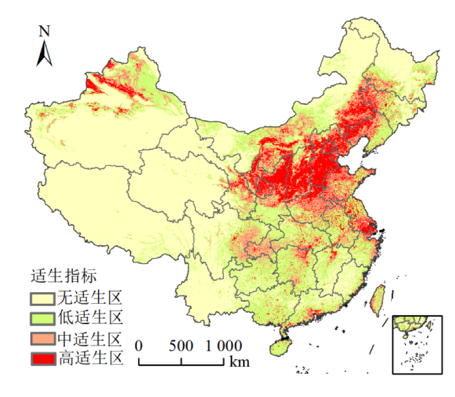
图6 当前反枝苋在中国的潜在适生区分布

Figure 6 Potential current and suitable area for A. retroflexus in China

图7 不同气候情景下反枝苋在中国的潜在适生区分布

Figure 7 Potentially suitable area distribution of A. retroflexus under different climate change scenarios in China

图8 未来气候变化情景下反枝苋的适生区变化

Figure 8 The suitable area changes of A. retroflexus under future climate change scenarios

表5 未来气候变化情景下反枝苋的适生区范围变化

Table 5 The scope change of A. retroflexus suitable area under future climate change scenarios 106 km2

气候变化情景	收缩区	扩张区	稳定区
2030s, SSPs1-2.6	0.192	0.490	4.20
2030s, SSPs2-4.5	0.185	0.539	4.21
2030s, SSPs5-8.5	0.091	0.634	4.30
2050s, SSPs1-2.6	0.270	0.579	4.12
2050s, SSPs2-4.5	0.245	0.745	4.15
2050s, SSPs5-8.5	0.259	0.938	4.14

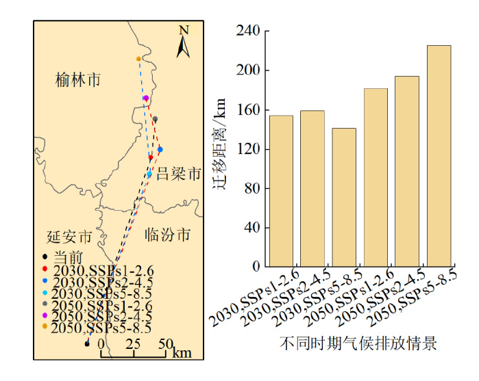
图9 不同时期反枝苋适生区分布重心及迁移距离

Figure 9 The distribution center of gravity and migration distance of A. retroflexus suitable area in different periods

参考文献 47

[1]	AHMED S E, MCINERNY G, O'HARA K, et al., 2015. Scientists and software-surveying the species distribution modelling community[J]. Diversity Distributions, 21(3): 258-267.
[2]	ALLOUCHE O, TSOAR A, KADMON R, 2006. Assessing the accuracy of species distribution models: Prevalence, kappa and the true skill statistic (TSS)[J]. Journal of Applied Ecology, 43(6): 1223-1232.
[3]	BELLARD C, THUILLER W, LEROY B, et al., 2013. Will climate change promote future invasions?[J]. Global Change Biology, 19(12): 3740-3748. DOI PMID
[4]	BOULANGEAT I, GRAVEL D, THUILLER W, 2012. Accounting for dispersal and biotic interactions to disentangle the drivers of species distributions and their abundances[J]. Ecology Letters, 15(6): 584-593. DOI PMID
[5]	BREIMAN L, 2001. Random forests[J]. Machine Learning, 45: 5-32.
[6]	BROGNIEZ D, BALLABIO C, STEVENS A, et al., 2015. A map of the topsoil organic carbon content of Europe generated by a generalized additive model[J]. European Journal of Soil Science, 66(1): 121-134.
[7]	BROWN J L, 2014. SDM toolbox: A python‐based GIS toolkit for landscape genetic, biogeographic and species distribution model analyses[J]. Methods in Ecology Evolution, 5(7): 694-700.
[8]	CHEN I C, HILL J K, OHLEMÜLLER R, et al., 2011. Rapid range shifts of species associated with high levels of climate warming[J]. Science, 333(6045): 1024-1026. DOI PMID
[9]	DICOLA V, BROENNIMANN O, PETITPIERRE B, et al., 2017. ecospat: An R package to support spatial analyses and modeling of species niches and distributions[J]. Ecography, 40(6): 774-787.
[10]	DINU M, ANGHEL A I, OLARU O T, et al., 2017. Toxicity investigation of an extract of Amaranthus retroflexus L. (Amaranthaceae) leaves[J]. Farmacia, 65(2): 289-294.
[11]	ELITH J, LEATHWICK J R, 2009. Species distribution models: ecological explanation and prediction across space and time[J]. Annual Review of Ecology, Evolution, and Systematics, 40: 677-697.
[12]	ELITH J, LEATHWICK J R, HASTIE T, 2008. A working guide to boosted regression trees[J]. Journal of Animal Ecology, 77(4): 802-813. DOI PMID
[13]	FANG Y Q, ZHANG X H, WEI H Y, et al., 2021. Predicting the invasive trend of exotic plants in China based on the ensemble model under climate change: A case for three invasive plants of Asteraceae[J]. Science of the Total Environment, 756: 143841.
[14]	FRIEDMAN J H, 1991. Multivariate adaptive regression splines[J]. The Annals of Statistics, 19(1): 1-67.
[15]	GASSÓ N, THUILLER W, PINO J, et al., 2012. Potential distribution range of invasive plant species in Spain[J]. NeoBiota, 12: 25-40.
[16]	GUO K Q, JIANG X L, XU G B, 2021. Potential suitable distribution area of Quercus lamellosa and the influence of climate change[J]. Chinese Journal of Ecology, 40(8): 2563-2574.
[17]	HAMAD A M, NELDER J A, 1997. Generalized linear models for quality-improvement experiments[J]. Journal of Quality Technology, 29(3): 292-304.
[18]	HANLEY J A, MCNEIL B J, 1982. The meaning and use of the area under a receiver operating characteristic (ROC) curve[J]. Radiology, 143(1): 29-36. DOI PMID
[19]	HAO Q, MA J S, 2023. Invasive alien plants in China: An update[J]. Plant Diversity, 45(1): 117-121.
[20]	HAO T, ELITH J, LAHOZMONFORT J J, et al., 2020. Testing whether ensemble modelling is advantageous for maximising predictive performance of species distribution models[J]. Ecography, 43(4): 549-558.
[21]	HASTIE T, TIBSHIRANI R, BUJA A, 1994. Flexible discriminant analysis by optimal scoring[J]. Journal of the American Statistical Association, 89(428): 1255-1270.
[22]	HULME P E, 2017. Climate change and biological invasions: evidence, expectations, and response options[J]. Biological Reviews, 92(3): 1297-1313.
[23]	LEK S, GUÉGAN J F, 1999. Artificial neural networks as a tool in ecological modelling, an introduction[J]. Ecological Modelling, 120(2-3): 65-73.
[24]	LI J Y, CHANG H, LIU T, et al., 2019. The potential geographical distribution of Haloxylon across Central Asia under climate change in the 21st century[J]. Agricultural Forest Meteorology, 275: 243-254.
[25]	LOPES A, DEMARCHI L O, PIEDADEM T F, et al., 2023. Predicting the range expansion of invasive alien grasses under climate change in the Neotropics[J]. Perspectives in Ecology Conservation, 21(2): 128-135.
[26]	NIX H, BUSBY J, 1986. BIOCLIM, a bioclimatic analysis and prediction system[M]. Division of Water Land Resources: Canberra.
[27]	PEARSON R G, DAWSON T P, 2003. Predicting the impacts of climate change on the distribution of species: Are bioclimate envelope models useful?[J]. Global Ecology Biogeography, 12(5): 361-371.
[28]	PETER A, ŽLABUR J Š, ŠURIĆ J, et al., 2021. Invasive plant species biomass-Evaluation of functional value[J]. Molecules, 26(13): 3814.
[29]	PHILLIPS S J, ANDERSON R P, DUDíK M, et al., 2017. Opening the black box: An open-source release of Maxent[J]. Ecography, 40(7): 887-893.
[30]	PHILLIPS S J, ANDERSON R P, SCHAPIRE R E, 2006. Maximum entropy modeling of species geographic distributions[J]. Ecological Modelling, 190(3-4): 231-259.
[31]	QIAO H J, LIN C T, JI L Q, et al., 2012. mMWeb-an online platform for employing multiple ecological niche modeling algorithms[J]. PLOS ONE, 7(8): e43327.
[32]	QIN Z, ZHANG J E, JIANG Y P, et al., 2018. Invasion process and potential spread of Amaranthus retroflexus in China[J]. Weed Research, 58(1): 57-67.
[33]	ROGER E, DUURSMA D E, DOWNEY P O, et al., 2015. A tool to assess potential for alien plant establishment and expansion under climate change[J]. Journal of Environmental Management, 159: 121-127. DOI PMID
[34]	SONG J Y, ZHANG H, LI M, et al., 2021. Prediction of spatiotemporal invasive risk of the red import fire ant, Solenopsis invicta (Hymenoptera: Formicidae), in China[J]. Insects, 12(10): 874.
[35]	TELEWSKIF W, ZEEVAARTJAJAJO B, 2002. The 120-yr period for Dr. Beal’s seed viability experiment[J]. American Journal of Botany, 89(8): 1285-1288.
[36]	THUILLER W, RICHARDSON D M, PYŠEK P, et al., 2005. Niche based modelling as a tool for predicting the risk of alien plant invasions at a global scale[J]. Global Change Biology, 11(12): 2234-2250.
[37]	VAYSSIÈRES M P, PLANT R E, ALLENDIAZ B H, 2000. Classification trees: An alternative non-parametric approach for predicting species distributions[J]. Journal of Vegetation Science, 11(5): 679-694.
[38]	WALTHER B A, PIRSIG L H, 2017. Determining conservation priority areas for Palearctic passerine migrant birds in sub-Saharan Africa[J]. Avian Conservation and Ecology, 12(1): 2.
[39]	WANG R, WANG Y Z, 2006. Invasion dynamics and potential spread of the invasive alien plant species Ageratina adenophora (Asteraceae) in China[J]. Diversity Distributions, 12(4): 397-408.
[40]	WENG Y W, CAI W J, WANG C, 2020. The application and future directions of the shared socioeconomic pathways (SSPs)[J]. Advances in Climate Change Research, 16(2): 215-222.
[41]	YE X Z, ZHAO G H, ZHANG M Z, et al., 2020. Distribution pattern of endangered plant Semiliquidambar cathayensis (Hamamelidaceae) in response to climate change after the last interglacial period[J]. Forests, 11(4): 434.
[42]	ZHU L W, CAO D D, HU Q J, et al., 2016. Physiological changes and sHSPs genes relative transcription in relation to the acquisition of seed germination during maturation of hybrid rice seed[J]. Journal of the Science of Food Agriculture, 96(5): 1764-1771.
[43]	李晓晶, 张宏军, 倪汉文, 2004. 反枝苋的生物学特性及防治[J]. 农药科学与管理, 25(3): 13-16.
	LI X J, ZHANG H J, NI H W, 2004. Review on the biological characters and control of redroot pigweed (Amaranthus retroflexus)[J]. Pesticide Science and Administration, 25(3): 13-16.
[44]	刘伟, 朱丽, 桑卫国, 2007. 影响入侵种反枝苋分布的环境因子分析及可能分布区预测[J]. 植物生态学报, 31(5): 834-841. DOI
	LIU W, ZHU L, SANG W G, 2007. Potential global geographical distribution of Amaranthus retroflexus[J]. Chinese Journal of Plant Ecology, 31(5): 834-841.
[45]	塞依丁·海米提, 2020. 气候变化情景下入侵种反枝苋在新疆的潜在分布格局研究[D]. 乌鲁木齐: 新疆大学.
	SEIDIN HAMID, 2020. Potential distribution pattern of invasive species Amaranthus retroflexus L. in Xinjiang under climate change[D]. Urumqi: Xinjiang University.
[46]	魏莹, 李倩, 李阳, 等, 2020. 外来入侵植物反枝苋的研究进展[J]. 生态学杂志, 39(1): 282-291.
	WEI Y, LI Q, LI Y, et al., 2020. Research advances of invasive alien plant Amaranthus retroflexus L.[J]. Chinese Journal of Ecology, 39(1): 282-291.
[47]	辛晓歌, 吴统文, 张洁, 等, 2019. BCC模式及其开展的CMIP6试验介绍[J]. 气候变化研究进展, 15(5): 533-539.
	XIN X G, WU T W, ZHANG J, et al., 2019. Introduction of BCC models and its participation in CMIP6[J]. Advances in Climate Change Research, 15(5): 533-539.

基于集合模型预测外来植物反枝苋的入侵趋势

Prediction of Invasive Trend of Alien Plant Amaranthus retroflexus Based on Ensemble Model

RichHTML

PDF

可视化

摘要/Abstract

引用本文

使用本文

图/表 14

参考文献 47

相关文章 1

编辑推荐

Metrics

本文评价